This tutorial is an overview of the philosophy behind different types of reconstruction algorithms for tomography. We are going to discuss their strengths and pitfalls when it comes to reconstructing tomography data. We won’t however go into the nuts and bolts of every specific reconstruction algorithm.
Ideally, at the end of this tutorial, you should have a high level overview of the main families of reconstruction algorithms, and be able to navigate the algorithm landscape to select the best option for your specific problem.
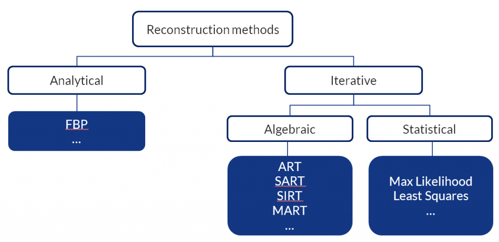
For the sake of this tutorial, we are going to divide the reconstruction algorithms into three families:
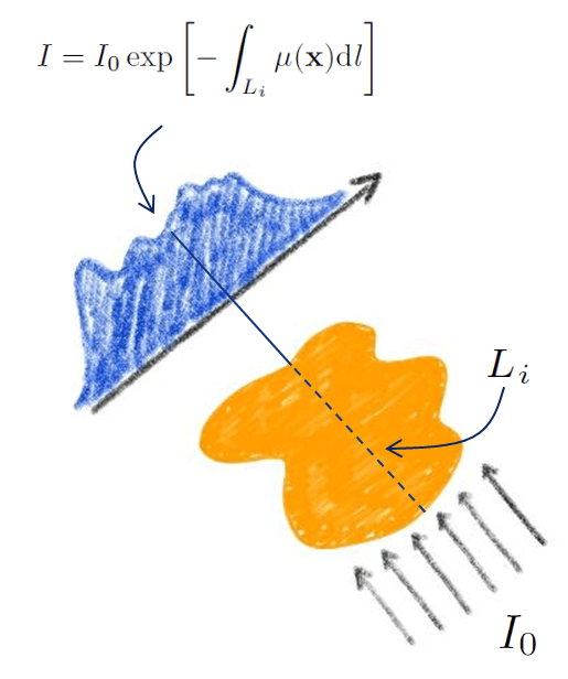
Filtered back-projection (FBP) is based on the measurement of transmitted (or emitted) intensity from a sample, that can be recast as a line integral of some sample property. For x-ray tomography this is typically the attenuation coefficient. We call this measured quantity the “projection“.
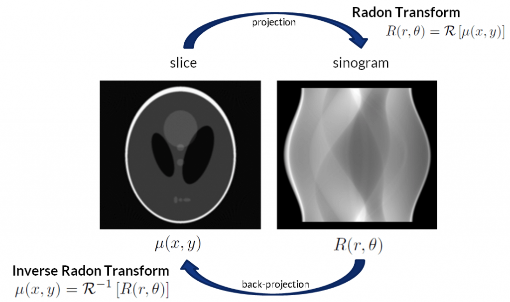
The essence of FBP is that the combination of all projections (commonly called the sinogram) is related to the attenuation coefficient by an exact mathematical operation, known as Radon Transform.
Never mind how complicated the Radon Transform may look like; the important thing to keep in mind is that such a transform does exist, it can be computed and, most importantly, can be inverted.
That’s right. In the FBP setting, tomographic reconstruction boils down to an “inverse Radon Transform” which means to numerically computing the inverse relation which goes from the sinogram (the thing we measure) to the virtual slice (the thing we would like to reconstruct).
Pros of FBP
Cons of FBP
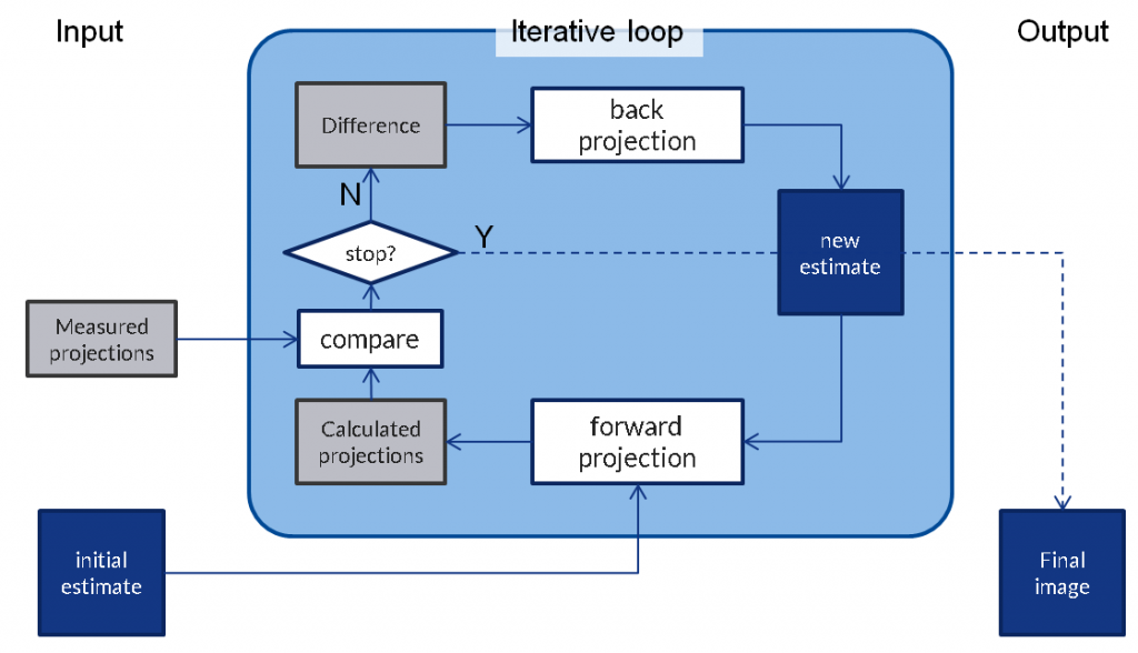
Algebraic reconstruction techniques (ART) group a family of algorithms that aims at solving the tomographic problem iteratively. In ART, the slice to be reconstructed is modelled as a discrete array of pixels (with unknown value) from the outset. Also, instead of considering an ideal line projection, ART accounts for the finite width of the resolution element by modelling an overlap between the ‘beam’ (i.e. the projection of the detector resolution element along the beam) and the pixel size in the plane of the slice.
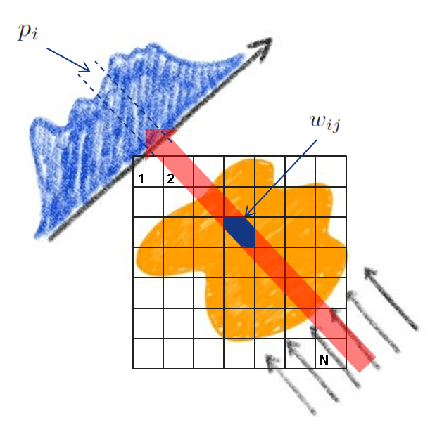
Look at the following figure: the beam does not cross all pixels equally, and the overlap of the beam with each pixel is modelled as a weight coefficient wij
In ART you can forget the Radon Transform. The projection pi on each detector element is simply the weighted sum of the rays that crossed the line of pixels in the slice: pi=∑j=1Nwijμj where μj is the value at the attenuation coefficient at the pixels j. Now, the equation above is in fact a massive system of equations: hundreds of thousands or even millions of equations are hiding in that tiny little equation. This is the main reason why trying to solve that system in closed form is pointless. In addition, given that you always have random noise, a solution to the system may not even exist, or if it does it may not be unique.
This figure above is adapted from adapted from M. Beister et al, Physica Medica 28, 94 (2012).
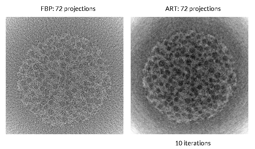
Here’s a comparison on a reconstructed data from a72 projections neutron tomography scan taken at the instrument DINGO, at the Australian Centre for Neutron Scattering, in Sydney. FBP reconstruction is shown on the left (almost no contrast). SART reconstruction run in Python is shown on the right. Contrast is much better after just 10 iterations.
Pros of ART
Cons of ART
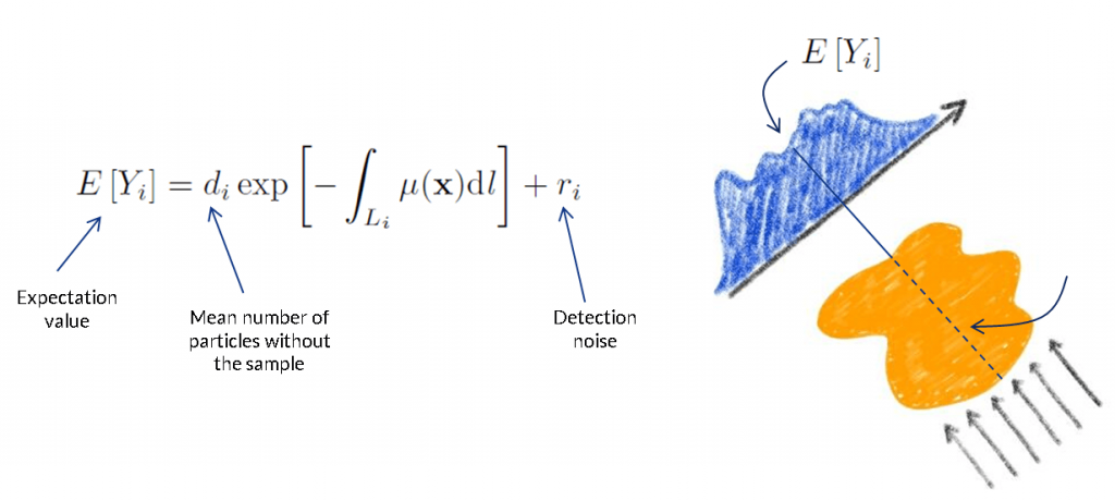
The key idea of statistical methods is to incorporate counting statistics of the detected photons/particles into the reconstruction process.
Statistical methods were initially developed for very low counting statistics typical of emission tomography schemes such as PET (I’ve put a few reference at the end of this article). In a nutshell, statistical algorithms are based on accurate modelling of the incoming particles or photons, interactions with the sample, and finally detection of these particles. All of these processes are ‘statistical’ in the sense that each individual process (for instance the absorption of an x-ray photon by a sample) is a stochastic process.
The whole description of detected intensity as a line integral (as in FBP) or ray sum over pixels (as in ART) is no longer appropriate for statistical methods. The detected intensity of particles after the sample becomes a random variable . All projections measurements are independent random variables whose expectation value is Yi.
My colleague Jeremy M.C. Brown has written some amazing code to perform statistical reconstruction, and we applied together on neutron tomography measurements. The reference to the paper is below. The take-home message of our work was that statistical methods reach comparable results to FBP with just about 12% of the projections required. That’s right, that is more than 80% saving in scan time (or radiation dose) for comparable results. By comparable we mean comparable signal-to-noise and resolution.
Pros of statistical methods
Cons of statistical methods
The topic of statistical reconstruction becomes very technical, very soon, and this is way outside the idea of this introductory tutorial. For those of you who are interested in learning a bit more on this topic, I recommend the following resources.
| Cookie | Duration | Description |
|---|---|---|
| cookielawinfo-checkbox-analytics | 11 months | This cookie is set by GDPR Cookie Consent plugin. The cookie is used to store the user consent for the cookies in the category "Analytics". |
| cookielawinfo-checkbox-functional | 11 months | The cookie is set by GDPR cookie consent to record the user consent for the cookies in the category "Functional". |
| cookielawinfo-checkbox-necessary | 11 months | This cookie is set by GDPR Cookie Consent plugin. The cookies is used to store the user consent for the cookies in the category "Necessary". |
| cookielawinfo-checkbox-others | 11 months | This cookie is set by GDPR Cookie Consent plugin. The cookie is used to store the user consent for the cookies in the category "Other. |
| cookielawinfo-checkbox-performance | 11 months | This cookie is set by GDPR Cookie Consent plugin. The cookie is used to store the user consent for the cookies in the category "Performance". |
| viewed_cookie_policy | 11 months | The cookie is set by the GDPR Cookie Consent plugin and is used to store whether or not user has consented to the use of cookies. It does not store any personal data. |