Segmentation is a common procedure for feature extraction in images and volumes. Segmenting an image means grouping its pixels according to their value similarity. For instance in a CT scan, one may wish to label all pixels (or voxels) of the same material, or tissue, with the same color. The simplified-color image (or volume) can then be used to render important features independently from one another (for instance bone from muscle).
Segmentation is essentially the same thing as color simplification or color quantization, used to simplify the color scale of an image, or to create poster effects. In this post we discuss how to segment a reconstructed slice from a micro-CT scan using k-means clustering.
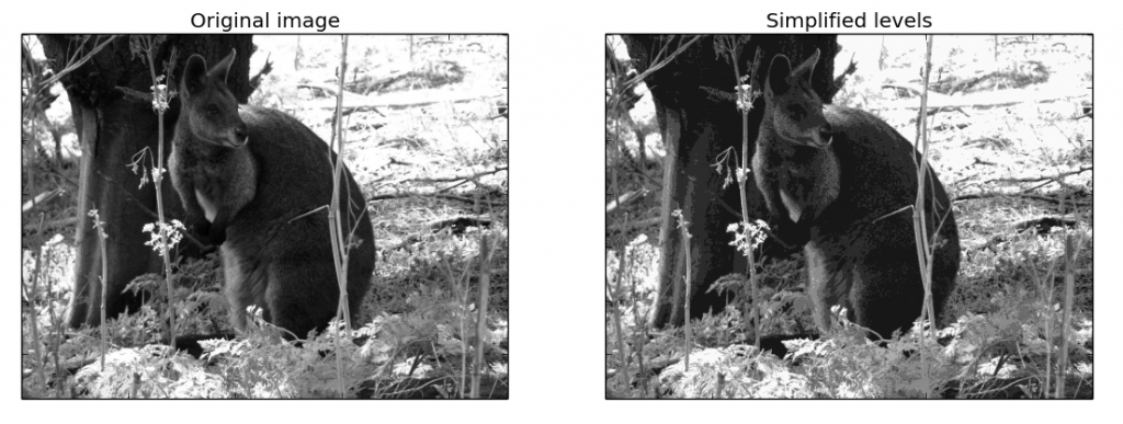
k-means clustering is a machine learning technique used to partition data. If your data consists of n observations, with k-means clustering you can partition these observations into k groups, according to some similarity rule. Let’s apply this idea to segmentation: if your image has n grey levels, you can group these into k intervals, according to how close they are together.
Let’s work through a simple example, using Scikit-Learn in Python. The snippet below opens a jpeg image from file and simplifies its colors to 8 grey levels. This example is inspired by the Vector Quantization Example available on the Scikit-Learn website.
#Source: Instruments & Data Tools
#Inspired from the Vector Quantization Example

from sklearn import cluster
from skimage import data
import numpy as np
import matplotlib.pyplot as plt

def km_clust(array, n_clusters):

    # Create a line array, the lazy way
    X = array.reshape((-1, 1))
    # Define the k-means clustering problem
    k_m = cluster.KMeans(n_clusters=n_clusters, n_init=4)
    # Solve the k-means clustering problem
    k_m.fit(X)

    # Get the coordinates of the clusters centres as a 1D array
    values = k_m.cluster_centers_.squeeze()

    # Get the label of each point
    labels = k_m.labels_

    return(values, labels)

# Read the data as greyscale
img = data.imread('roo.jpg',as_grey=True)

# Group similar grey levels using 8 clusters
values, labels = km_clust(img, n_clusters = 8)

# Create the segmented array from labels and values
img_segm = np.choose(labels, values)
# Reshape the array as the original image
img_segm.shape = img.shape

# Get the values of min and max intensity in the original image
vmin = img.min()
vmax = img.max()

fig = plt.figure(1)
# Plot the original image
ax1 = fig.add_subplot(1,2,1)
ax1.imshow(img,cmap=plt.cm.gray, vmin=vmin, vmax=vmax)
ax1.set_title('Original image')

# Plot the simplified color image
ax2 = fig.add_subplot(1,2,2)
ax2.imshow(img_segm, cmap=plt.cm.gray, vmin=vmin, vmax=vmax)
ax2.set_title('Simplified levels')

# Get rid of the tick labels
ax1.set_xticklabels([])
ax1.set_yticklabels([])
ax2.set_xticklabels([])
ax2.set_yticklabels([])

plt.show()
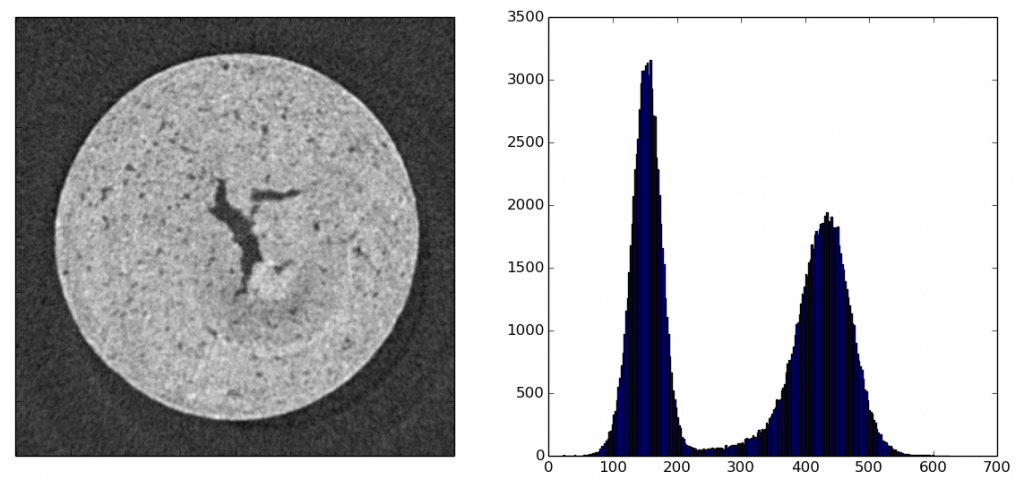
Well, the same idea can be applied to image segmentation. We’ll use a reconstructed slice from a micro-CT scan. In tomography (CT or OPT) the grey levels are related to some physical quantity in our data, for instance optical density. Therefore segmentation enables quantitative imaging of these properties.
OK, enough said, let’s modify our code to deal with an image representing a slice reconstructed from a CT scan of a porous material.
# Read the data as greyscale
img = data.imread('porous_material.tif',as_grey=True)
# Reshape as 1D array
img_flat = img.reshape((-1, 1))

fig = plt.figure(1)

ax1 = fig.add_subplot(1,2,1)
ax1.imshow(img,cmap=plt.cm.gray)

ax2 = fig.add_subplot(1,2,2)
# Plot the histogram with 256 bins
ax2.hist(img_flat,256)

ax1.set_xticklabels([])
ax1.set_yticklabels([])

plt.show()
Let’s look at the histogram: the peak on the left is the noise, the one on the right corresponds to the grey levels of the sample image. So, first we want to separate signal from noise, then segment the signal.
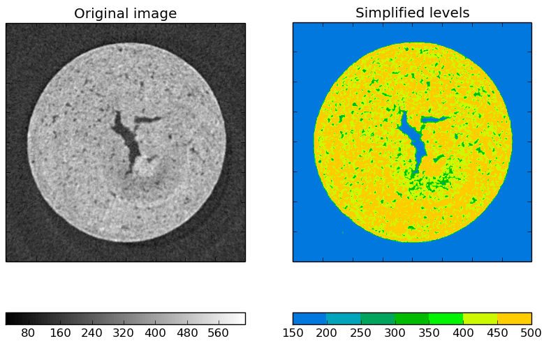
We apply the snippet above and this is what we get. The blue is used for the noise (empty space and voids) and the other levels for different density or composition in the sample.

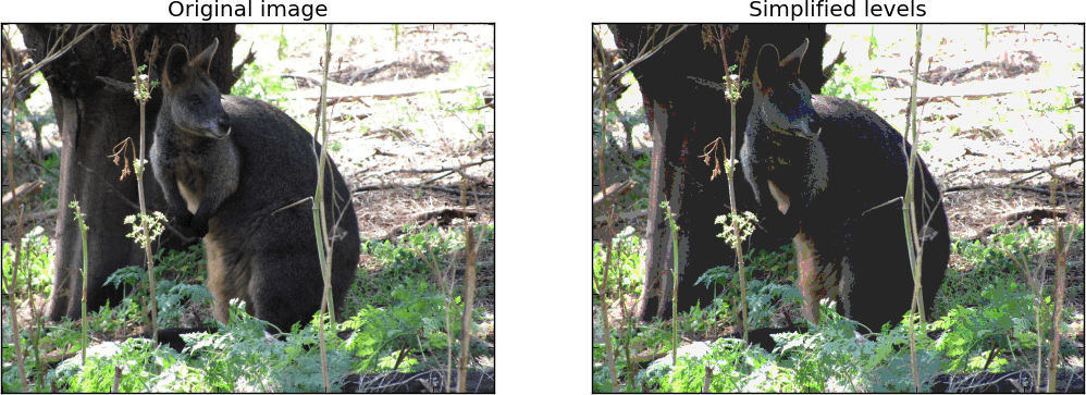
Before wrapping up, let’s take a quick look at how to use our snippet to posterize an RGB image. We’ll use the kangaroo photo we used before.Quite surprisingly, we just need a couple of small changes to the code to make this work.
The first, obviously, is to open the image as an RGB.
# Read the data as RGB
img = data.imread('roo.jpg')
The second thing to do is to convert the data in 8-bit when we create the segmented array from labels and values
# Create the segmented array from labels and values
img_segm = np.choose(labels, values).astype('uint8')
The last step is required because an RGB image contains three channels of 8-bit data, ranging from 0 to 255. If we don’t convert to 8-bit the that the results will be nonsense (a funky looking kangaroo, give it a try). Having 16 (or more) bit in a grayscale image is not a problem and hence we didn’t need to bother to convert a grayscale image to 8-bit.
Anyway, here’s the result.

There are couple of more things we can still do with our data, let’s just list a couple for future reference:
Well that’s it for this post. Thanks for reading.
| Cookie | Duration | Description |
|---|---|---|
| cookielawinfo-checkbox-analytics | 11 months | This cookie is set by GDPR Cookie Consent plugin. The cookie is used to store the user consent for the cookies in the category "Analytics". |
| cookielawinfo-checkbox-functional | 11 months | The cookie is set by GDPR cookie consent to record the user consent for the cookies in the category "Functional". |
| cookielawinfo-checkbox-necessary | 11 months | This cookie is set by GDPR Cookie Consent plugin. The cookies is used to store the user consent for the cookies in the category "Necessary". |
| cookielawinfo-checkbox-others | 11 months | This cookie is set by GDPR Cookie Consent plugin. The cookie is used to store the user consent for the cookies in the category "Other. |
| cookielawinfo-checkbox-performance | 11 months | This cookie is set by GDPR Cookie Consent plugin. The cookie is used to store the user consent for the cookies in the category "Performance". |
| viewed_cookie_policy | 11 months | The cookie is set by the GDPR Cookie Consent plugin and is used to store whether or not user has consented to the use of cookies. It does not store any personal data. |